


Comparing drone UAV LiDAR and Photogrammetry
In this article we will be comparing drone UAV LiDAR and Photogrammetry. Drones are emerging as a useful tool for survey applications. Drones are often fitted with cameras for survey, and thus to perform photogrammetry, or – less frequently – with laser scanners for LiDAR. This paper provides a comparison between these two methods at a test location, with a common goal, the generation of a Digital Terrain Model (DTM) of the area. It is known that the selection of the method should be highly dependent on the intended application. For the testcase presented below, the analysis of the results show that photogrammetry was more accurate – both DTM accuracy and vertical absolute accuracy – than LiDAR in this built terrain.
Introduction
Drones have proven to be a revolutionary technology in the field of surveying and mapping. Their flexible and cost-efficient nature as well as the high-resolution end-products make them increasingly appealing to surveyors. As a result, more and more surveying companies acquire their own fleet of drones. Apart from the higher quality of data they provide when compared to most other airborne methods, due to the much lower flying heights, drones contribute significantly to the risk reduction. drones make it possible to perform high risk tasks in a safe manner, such as inspections in dangerous areas.
The two most popular methods for capturing terrain information using a drone are (aerial) photogrammetry and (airborne) LiDAR (Light Detection And Ranging). Photogrammetry is based on performing measurements on overlapping photographs for the extraction of 3D information. It is a passive remote sensing technique since the main instrument used is a camera. On the other hand, LiDAR uses an active sensor, the laser scanner, and thus it belongs to active remote sensing. It is a ranging technique, which means that distances to a target surface are measured by illuminating it with a pulsed laser light and measuring the reflected pulses with a sensor. Because of the differences in the measuring principles of these two methods, there are advantages and disadvantages depending on the application. LiDAR versus photogrammetry has recently become a subject of continuous discussions in the aerial surveying community.
LiDAR is commonly regarded as superior to photogrammetry because vegetation can be penetrated, ground control points are no longer needed, and processing times are shorter. However, photogrammetry can typically achieve high data quality in a much more cost-efficient way when compared to LiDAR. This means that both methods can provide us with high accuracies, but for LiDAR the investment for the instruments is significantly larger. When it comes to vegetated areas LiDAR excels over photogrammetry, due to its ability to penetrate through vegetation. The same happens when surveying narrow objects (e.g. transmission lines, pipelines, sharp-edge features). Another major difference between the two methods is the need for Ground Control Points (GCPs). In most cases, photogrammetry is based on the existence of GCP’s for the correct reconstruction of the model. The only case that GCP’s would not be necessary is if the flight positions of the UAV were known using the GPS Post-Processed Kinematic (PPK) method. These positions would correspond to all the positions where the camera triggered. On the contrary, LiDAR is totally independent of them. With LiDAR additional measured points are used only for validation purposes. These and other differences led Skeye to the initiative of comparing the two methods in the same project area and for the same application.
The Project
The breakwater in Scheveningen, in the Netherlands, was chosen as the test location for the comparison of the two methods (see Figure 1). This breakwater was also part of the BREAKWATERHEALTHSCAN® joint initiative, more information about which can be found in its official website (www.breakwaterhealthscan.com).

For the photogrammetric survey, an Altura Zenith ATX8 drone was used in combination with a Sony Alpha ILCE-7R full-frame camera (using 28 mm focal length). The flying height was 50 meters Above Ground Level (AGL) and the forward and side overlap were both 80%. With this configuration three flights were performed during which 585 images with a Ground Sampling Distance (GSD) of 9 mm were captured. For that survey, 26 GCPs and 16 check points (CHPs) were measured using RTK GNSS and, validated with more traditional levelling.
For the LiDAR survey, the same drone was used, but this time in combination with the aerial LiDAR system YellowScan Surveyor (see Figure 2). This system consists of the Velodyne VLP-16 (Puck) laser scanner and the Trimble APX-15 UAV GNSS-Inertial system by Applanix. Table 1 is an overview of YellowScan Surveyor’s main specifications.

From the table, we can conclude to that, although the range is a limiting factor – since we cannot fly higher than 50 m AGL, this system can provide us with a high-density point cloud due to its high scan rate. In addition, the UAV flights can be longer since it weighs only 1.6 Kg. With this system, three flights were performed, covering almost the same area (the breakwater) but with different flight plans each time. The flying height was common for all three of them and equal to 30 meters AGL. This height was chosen to be lower than the one of the photogrammetric flight to increase the point density (since the shape of the survey area allowed us to do so, being narrow and long). For the geo-referencing of the derived point cloud with the method of RTK, a GNSS base station was set up in the project area.

Drone LiDAR A priori accuracy estimation
To get a measure of the absolute accuracy – thus with respect to the ground truth data – that can be achieved, an a priori accuracy estimation was performed for both the photogrammetry and LiDAR system. Starting with photogrammetry, the literature combined with our experience suggests that the absolute vertical accuracy that can be achieved is between 1 to 3 times the GSD. In this test case, the GSD was 9 mm, so the expected accuracy is between 9 and 27 mm. It should be noted, though, that these values are valid only when the model is correctly reconstructed photogrammetrically.
For the estimation of the expected accuracy of the LiDAR, a motion error model was used. This model (see Figure 3) considers the geometry of each laser scanning measurement and the way that each different component of the LiDAR system contributes to the total error budget.

For the YellowScan Surveyor system, and by assuming zero attitude angles, the a priori 3D accuracy is calculated as:
| mX | 29 mm |
| mY | 36 mm |
| mZ | 35 mm |
So, the expected vertical accuracy for LiDAR is equal to 35 mm.
What follows is the presentation of the results derived from processing, which allow us to find out how close we can get to the expected accuracies.
Comparing results between drone LiDAR and photogrammetry
The processing of the photogrammetric dataset resulted in a Digital Terrain Model (DTM) and an orthophoto. The achieved point density of the photogrammetric point cloud was approximately 3500 points/m2. Figure 4 is a closer look at a small part of the DTM, aiming at depicting the high level of detail contained in this model with a grid size of 2 cm.

As Figure 4 illustrates, this model is characterised by smooth and clean surfaces, clear breaklines and no data gaps. In addition, Figure 5 shows a similar view of the orthophoto, with a resolution of 1 cm. With such a resolution, even the smallest features can be distinguished.

To validate the correctness of the products a quality control was performed based on the DTM and the measured check points, as presented in Table 2. However, as we will see later, the grid size of the DTM derived from the LiDAR point cloud was 5 cm. So, in order to have a fair comparison, the quality control of the photogrammetric DTM was also performed on a DTM of 5 cm grid size. That showed us that both the relative (with respect to the dataset itself) and the absolute accuracy is equal to 4 mm. Check points do not participate in the processing and thus they serve only for quality control purposes. The magnitude of the absolute accuracy is highly dependent on the quality of the measurements of the check point. Since the check points were measured using levelling, with an accuracy of 1-2 mm, the absolute accuracy that we could achieve was significantly higher than by using RTK GNSS.
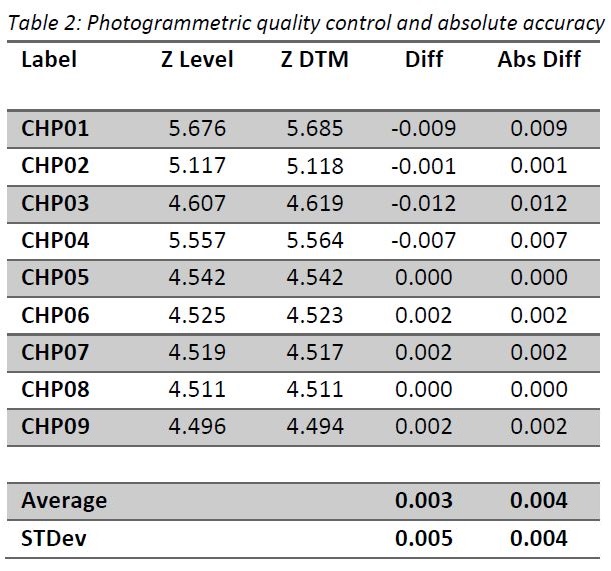
For calculating the accuracy, we prefer to use the absolute values of the height differences. If this was not the case, the errors could be averaged out (i.e. assume 10 heights to be 1 metre below and 10 heights 1 metre above the levelled heights).
The processing of the LiDAR dataset was considerably quicker (approximately 4 hours vs. 8 hours needed for the photogrammetric dataset). The main product was the DTM of the denoised point cloud. For this test, the point clouds of two (out of the three) flights were merged into a single point cloud to increase the point density. Merging all three point clouds would result in a much larger amount of points – that would make the dataset difficult to process – so the two with the highest precision (standard deviation between the points of one flight) were chosen. An average point density of 625 points/m2 was then achieved and consequently a DTM with a grid size of 5 cm was generated. This implies that in a simplified case of 400 points/m2 that are equally distributed the value that is assigned to each grid cell is derived from one single point. A grid size of 10 cm would also have been a good choice, since a minimum point density of 100 points/m2 (equally spaced) would have been required. But although usually the larger the grid size, the less data gaps, a decrease in the resolution is accompanied by a decrease in the absolute accuracy. Figure 6 is a close look of a small part of this DTM.

It is observed that the surfaces in this DTM are less smooth than in the DTM coming from photogrammetry. Using a different interpolation method, the result can be smoother but then we would deviate more from the true values. In addition, there are some data gaps due to the presence of water.
Using the GCP’s and the check points measured during the photogrammetric survey in combination with the DTM, a quality control was performed, and the absolute accuracy of the LiDAR dataset was found to be 20 mm (see Table 3).

It can be noticed that the number of check points in Table 3 is higher than in Table 2. That is because for the LiDAR validation some of the GCP’s used for the photogrammetric dataset could also be used. In addition, as it was also mentioned earlier, this accuracy was higher than expected due to the very high accuracy in determining the coordinates of the GCP’s and the check points.
Conclusions
UAV photogrammetry and LiDAR are the two methods that are expected to dominate the survey market in the future. We compared the two methods by performing a test at the breakwater in Scheveningen having as a main goal the generation of an accurate DTM of the surveyed structure. By processing the two datasets and comparing their results we found the following
- At first, the processing time needed for the DTM generation was significantly lower for the LiDAR dataset than for the photogrammetric one.
- With photogrammetry we achieved higher DTM resolution (2 cm versus 5 cm that was achieved with LiDAR). Higher level of detail is thus provided, something that can be very useful in certain applications that would require that.
- The DTM derived from the LiDAR dataset was less smooth when compared to the one derived from photogrammetry. That can be explained by the fact that, although the LiDAR point cloud was quite dense, the point distribution was not homogenous, since it depends a lot on the incidence angle of the scans.
- Photogrammetry provided us with a very high vertical accuracy (4 mm) thanks to, apart from the others, the high overlap in the images and the very low uncertainty in the GCPs’ and check points’ measurements.
- The vertical accuracy of LiDAR was also quite high (20 mm), considering the specifications of the LiDAR system used – the nominal accuracy is 5 cm, and is very close to the upper limit of the accuracy that can be achieved with LiDAR.
In general, none of the two methods can be regarded as better than the other one. In a built environment (like our test location), photogrammetry is preferable for the reasons mentioned above. On the other hand, though, in a vegetated area or for surveying narrow structures LiDAR is undoubtedly a more suitable solution. Therefore, the choice of the method should be made each time based on the nature of the project area and the requirements.
References
Peng, T., Lan, T., & Ni, G. (2013). Motion error analysis of 3D coordinates of airborne LIDAR under typical terrains. Measurement Science and Technology, 24(7).
Author
Chara Chatzikyriakou
Project Manager at Skeye B.V.
Co-author
Patrick Rickerby
Technical Director at Skeye Ltd.


